Predicted-Latency Based Scheduling for LLMs

Not all LLM requests cost the same. A short prompt might complete in milliseconds, while a long one can occupy a GPU for seconds. If we can predict how long a request will take on each candidate server before dispatching it, we can make substantially better routing decisions. This post describes a system that does exactly that: a lightweight ML model trained online from live traffic that replaces manually tuned heuristic weights with direct latency predictions.

The Load Balancing Problem in LLM Serving

The variation in request cost comes from how LLM inference works. It happens in two phases: first, the model processes the entire input prompt (the prefill phase), which is compute-heavy and scales with prompt length. Prefill can be accelerated when the server has already cached results from a similar prompt (prefix caching). Then it generates output tokens one at a time (the decode phase), which is memory-heavy and scales with the number of tokens generated.

Current load balancers try to account for this using signals like queue depth, memory pressure, cache locality, and batch size. But these signals often conflict: routing for cache reuse concentrates load, while routing for low utilization spreads it. Getting the balance right requires manual tuning of weights (see NVIDIA Dynamo or Inference Gateway), and the right balance shifts as the workload varies.

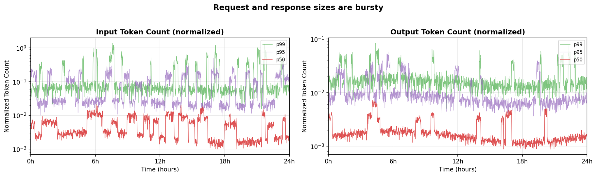
Production traffic makes this concrete. Figures below show metrics from an internal Google service serving an open model over 24 hours, patterns representative of what we see across production LLM deployments.

• Request and response sizes are bursty and have huge variance: Input and output token counts swing by orders of magnitude over the course of hours, driven by traffic that arrives in waves rather than at a steady rate. (Token counts are normalized by the model's maximum context length.)

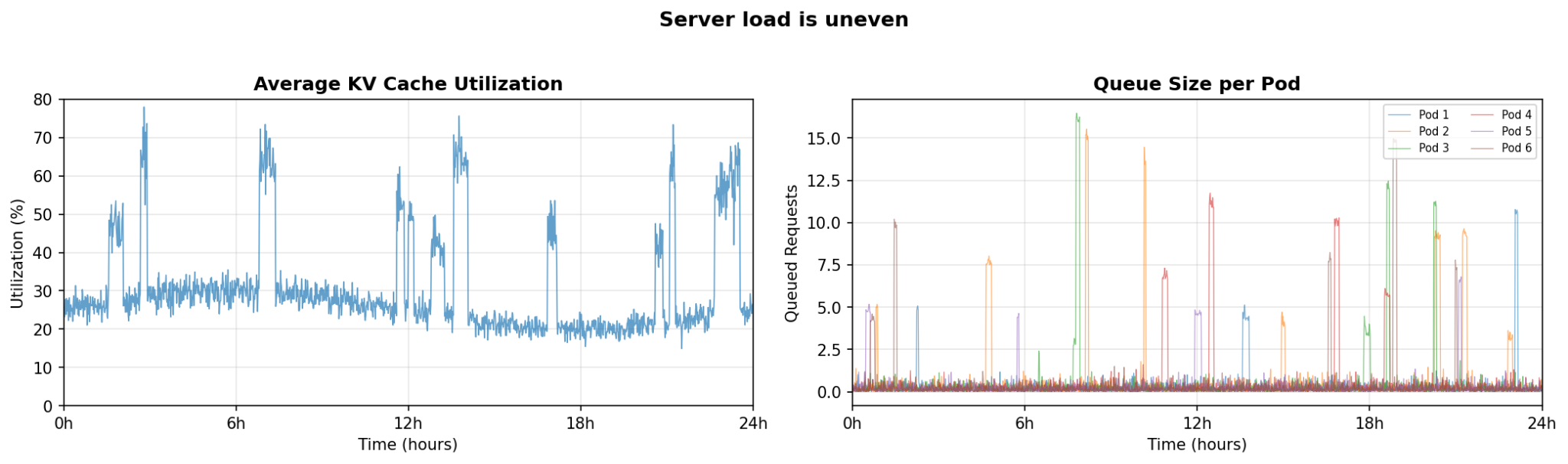
• Server load is uneven: These bursts hit servers differently. KV cache utilization (a measure of how much GPU memory is occupied by in-flight requests) spikes from 30% to over 70%. Queue depths spike just as unevenly.

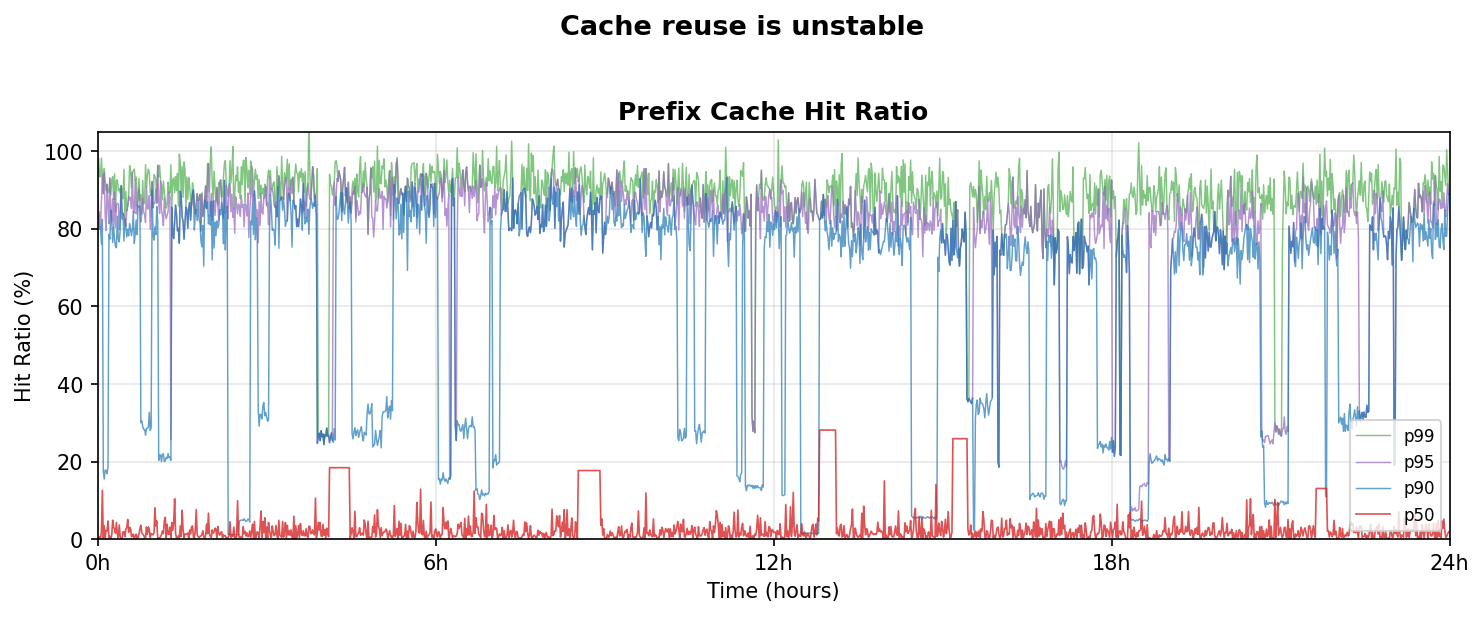
• Cache reuse is unstable: LLM servers cache previously computed results so that repeated prefixes (like a shared system prompt) don't need to be recomputed. Most requests see little to no cache reuse, while a subset benefits from high hit rates. But even that subset is unstable: hit rates collapse frequently as traffic patterns shift and cached prefixes get evicted. A load balancer tuned for high cache reuse will routinely encounter requests where that assumption doesn't hold.

These patterns are consistent with observations across production LLM deployments. Azure inference traces show significant variation in request sizes and heavy-tailed token distributions over short time windows [Stojkovic et al., "DynamoLLM," HPCA 2025]. BurstGPT documents burstiness and diversified concurrency patterns across 10.31 million traces from Azure OpenAI services [Wang et al., "BurstGPT," 2024].

No fixed configuration can handle this. Weights tuned for high cache reuse cause latency violations during cache misses, and weights tuned for worst-case reuse waste capacity when caching is working well.

Predicted-Latency Aware Scheduling

The two phases of LLM inference each have a standard latency metric: Time to First Token (TTFT) measures how long prefill takes, and Time Per Output Token (TPOT) measures how long each subsequent token takes to generate.

We train a lightweight XGBoost regression model in real-time on the relationship between request and server characteristics -- prompt length, prefix cache hit rate, number of running requests, queue depth, KV cache utilization -- and the observed TTFT and TPOT for completed requests. The model learns to approximate the underlying performance behavior of the model server and accelerator hardware, continuously retraining on a sliding window of recent data to track shifting workload patterns.

At scheduling time, the model predicts the TTFT and TPOT a new request would experience on each candidate server, given that server's current state. The scheduler then routes the request to the server with the best predicted outcome. When SLOs are provided, the scheduler prefers servers with positive headroom (predicted latency below the SLO); otherwise, it simply picks the server with the lowest predicted latency.

This largely eliminates manual weight tuning. Rather than deciding how much to value cache locality versus queue depth versus memory pressure, the model learns those tradeoffs directly from observed latency data.

Across five benchmark scenarios ranging from cache-friendly to cache-intensive workloads, predicted-latency aware scheduling outperforms or matches load+prefix-aware routing in four out of five cases. Additionally we achieve 43% improvement in P50 end-to-end latency on a representative MaaS workload, with 70% improvements in TTFT.

How It Works

Design Goals

The predicted-latency approach improves on utilization-based balancing in two key ways:

• Balancing spread vs consolidation under changing traffic: Minimizing TPOT requires spreading load to reduce batch size, while minimizing TTFT benefits from consolidation to maximize prefix cache reuse. The optimal balance between these strategies shifts as traffic patterns change. Utilization-based balancers rely on manually tuned weights to make this tradeoff, and any fixed configuration will be wrong as the workload varies. The predicted-latency model learns the relationship between server state, request characteristics, and actual latency outcomes, allowing it to dynamically balance between spreading and consolidation as conditions change.

• Best-fit scheduling in the presence of SLOs: When requests have latency SLOs, the optimal strategy is best-fit: pack requests into servers that can still meet SLO targets, keeping other servers free for future requests with higher GPU requirements. Utilization-based balancers have no way to determine whether a server can meet a request's SLO, they only see proxy signals like queue depth and memory pressure. The predicted-latency model directly estimates TTFT and TPOT per server, allowing the scheduler to compute headroom against SLO targets and route accordingly. This best-fit strategy can be especially useful with a heterogeneous pool of model servers (say a mix of H100 and B200 GPUs).

Predicting TTFT and TPOT

We use an XGBoost regression model that takes request and server state as input and outputs predicted TTFT and TPOT. The model was designed to be fast, accurate, pluggable, and able to learn online as workload characteristics shift.

Features

We assume all pods use the same accelerator class, a simplification that can be addressed in the future. Beyond that, load and request shape drive most of the variation in TTFT and TPOT.

Feature	What It Captures	Why It Matters
KV Cache Usage %	How full the decode state is	High KV cache -> higher TPOT and slower TTFT when memory is saturated
Input Length	Weight of the prefill step	Longer prompts -> higher prefill cost -> higher TTFT
Queue Depth	Backlog before scheduling	More waiting requests -> higher TTFT; correlates with prefill interruptions -> affects TPOT
Running Requests	Active GPU concurrency	Higher concurrency -> higher TTFT; larger decode batches -> higher TPOT
Prefix Cache Match %	How much KV reuse is possible	High match -> faster prefill -> lower TTFT; low match -> full attention -> higher TTFT
Input Tokens In Flight	Input tokens dispatched but not yet prefilled, plus input tokens already prefilled but still occupying KV cache (request not complete)	Captures both incoming prefill pressure and lingering memory footprint -> higher TTFT; helps the model anticipate load before it hits the server

Training Data

Performance characteristics in LLM serving are batch-dependent and shift too quickly for long-term historical averages to remain meaningful. To stay aligned with real traffic, the model:

• Collects the most recent samples using a sliding window
• Stratifies them into coarse buckets (KV cache % in steps of 10, prefix hit rate in steps of 0.25, etc.)
• Continuously retrains on this stratified dataset

Bucketing with a sliding window is important because it maintains samples from regimes that aren't showing up in the latest traffic. Without bucketing, a single global sliding window would let the newest data overwrite everything. For example, if current traffic sits around 60% KV cache utilization, older samples from 30% KV cache would eventually disappear -- and the model would forget how to predict in that regime.

Request Scheduling

The latency predictor runs as a sidecar to the Inference Gateway Endpoint Picker (EPP), hosting both training and prediction servers:

• Training server: Continuously trains the model from live traffic, sampling data across KV cache, queue states, and prefix scores to maintain a stratified training dataset. As new requests complete, it refreshes the dataset and retrains the TTFT/TPOT models.
• Prediction servers: Serve the trained models, returning predicted TTFT and TPOT given the current server load and request features.

We added a predicted-latency scorer to the EPP. The scorer compares predicted latencies to per-request SLOs and computes headroom (predicted latency minus SLO target). It then gives higher scores to servers with positive headroom, packing requests into servers that can still meet SLOs while keeping other pods free for future requests. If no SLOs are provided, it simply prefers servers with lower predicted latencies.

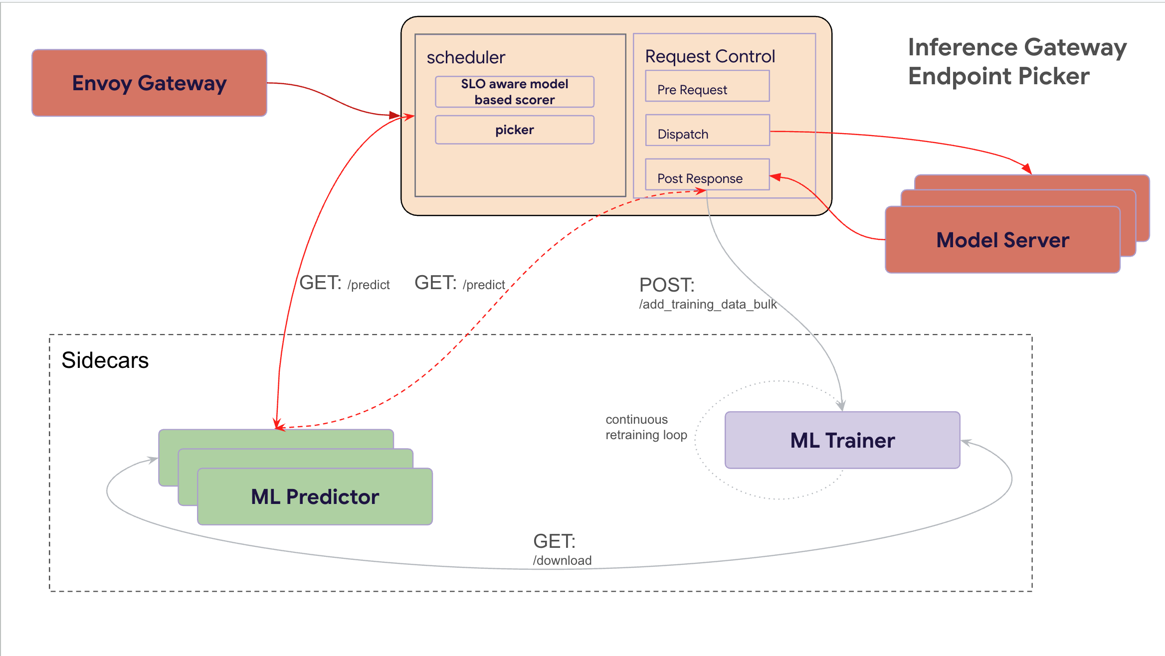
The predicted-latency trainer and predictor modules are deployed as sidecars to the EPP. The trainer is invoked at the post-response stage. The predictor is invoked during scheduling and optionally at the post-response stage. A new predicted-latency scorer utilizes predictions from the ML model.

Prediction Accuracy

Below we show predicted vs actual TTFT and TPOT over a benchmark run (scenario C below) as QPS increases stepwise toward saturation.

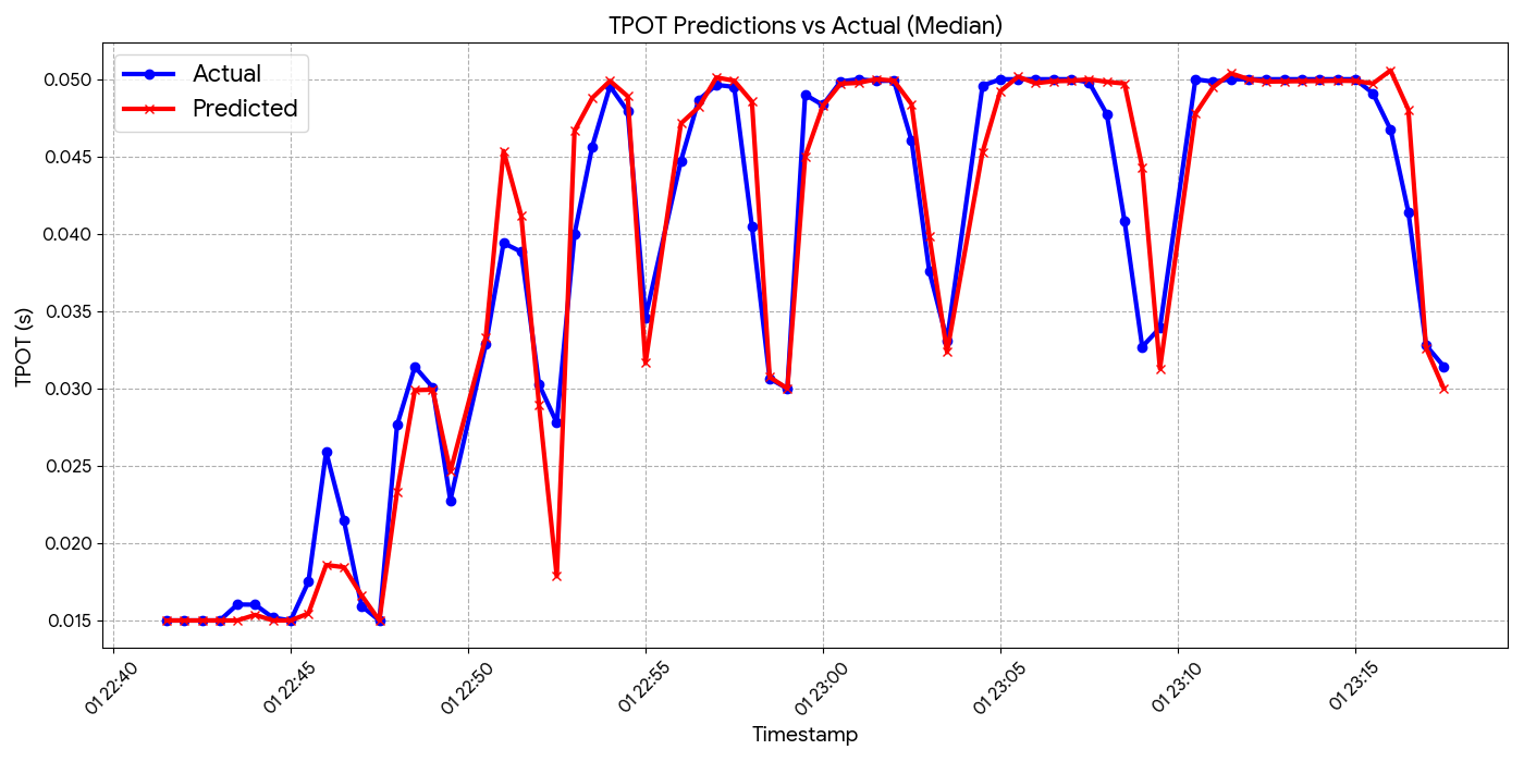
Predicted (red) vs actual (blue) TPOT over time. The model tracks steady-state TPOT well, even at transient spikes.

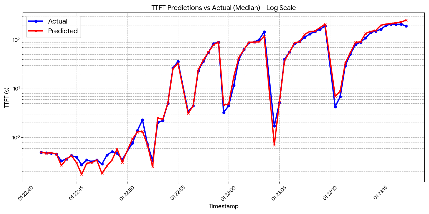
Predicted (red) vs actual (blue) TTFT over time. The model tracks TTFT closely as it ramps from near zero to 5 minutes across increasing QPS levels.

Across multiple benchmark runs, the model achieves a Mean Absolute Percentage Error (MAPE) of approximately 5%. This is not surprising -- accelerator performance is fairly deterministic given the current server state and request characteristics. The same prompt length, at the same KV cache utilization, with the same number of running requests, will produce similar TTFT and TPOT. The model simply learns this mapping.

Endpoint Selection

Given accurate TTFT and TPOT predictions, there are multiple possible algorithms for choosing the optimal endpoint -- for example, optimization-based approaches or multi-armed bandit strategies. We chose a greedy approach for its simplicity and low overhead, combined with a cache-aware affinity gate to prevent fragmentation.

Latency-based scoring. When SLOs are provided, the scorer computes headroom for each candidate server: how much room remains before the predicted latency exceeds the SLO target. To combine TTFT and TPOT into a single headroom score, we use a weighted combination -- by default 80% TTFT and 20% TPOT -- reflecting that TTFT is typically the more constraining metric in practice. The scheduler then does best-fit: it routes to the server with the least positive headroom, packing requests into servers that can still meet SLOs while keeping other servers free for future requests. When no SLOs are provided, the scorer simply routes to the server with the lowest predicted latency (most room).

Cache-aware affinity gate. Pure greedy routing can be counterproductive: a pod with no load but no cached prefix may have a lower predicted latency right now, but routing there means paying the full prefill cost and abandoning the cache built up on another pod. Over many requests, this leads to cache fragmentation -- prefixes are scattered across pods, no pod builds deep cache reuse, and the cluster loses the latency benefit of caching altogether. The opposite extreme is equally harmful: always routing to the pod with the best cache match concentrates popular prefixes on a few pods, which collapse under memory pressure.

To balance cache exploitation with exploration, the scorer uses an epsilon-greedy affinity gate:

• Exploit (99%): Filter candidates to pods whose prefix cache score exceeds a threshold (affinityGateTau, default 0.80). Among these, select the pod with the best predicted latency. Because the latency model already credits the cache benefit, this naturally picks the pod where cache reuse translates into actual lower latency, not just the highest raw cache score.

• Explore (1%): With probability epsilonExploreSticky (default 0.01), ignore the affinity gate entirely and consider all pods. These seeds cache entries on non-sticky pods, ensuring the cluster maintains cache diversity. Over time, these seeded entries grow into viable affinity targets, preventing the system from collapsing into a few overloaded cache-hot pods.

• Load gate: Even in the exploit path, if the best sticky pod's predicted TTFT exceeds the best overall pod's TTFT by more than affinityMaxTTFTPenaltyMs (default 5000ms), affinity is broken. This catches the case where queueing cost on a cache-hot pod has grown to outweigh the cache benefit, the predictor's latency estimate makes this comparison possible without manual thresholds on queue depth or memory.

The default threshold of 0.80 comes from production observation: prefix cache scores follow a bimodal distribution, roughly half of request-pod pairs have very high cache match (>0.80) and half have low match (<0.80). This reflects how prefix caching works in practice: in multi-turn conversations, a pod either has the conversation history cached from prior turns or it doesn't. Partial matches from unrelated conversations contribute very little because caching is block-based. The 0.80 threshold cleanly separates these two populations, so the affinity gate routes to pods that genuinely have your conversation cached rather than pods with incidental partial matches.

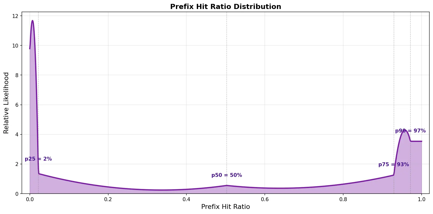
A typical production prefix hit ratio distribution observed in internal workloads, showing the bimodal pattern that motivates the 0.80 affinity threshold.

Benchmark Scenario Comparison

The table below contrasts five scenarios, ranging from cache-friendly (high prefix-sharing) to cache-intensive scenarios. We used the inference-perf library to enable shared prefix benchmarking configurations with multi-turn chat support. See Appendix for a complete analysis of the workloads.

Load Balancing Scorers

• Predicted Latency Scorer

• Load+Prefix Scorer: Combines pod load metrics (KV cache utilization and queued requests) with prefix cache awareness, balancing between resource utilization and cache locality.

  • Load metrics: KV cache utilization and queued request count
  • Prefix cache awareness: Considers cached prefix availability

  The set of weights used was: (1, 1, 1) prefix scorer: 1, queue scorer: 1, kv cache scorer: 1

• K8s Default Load Balancer: Standard Kubernetes round-robin or least-connection load balancing without cache or latency awareness (baseline).

Note that Predicted Latency Scorer eliminates the need to manually tune relative weights between different scoring components, as the ML model learns optimal trade-offs from historical data.

---

Hardware Configuration: 10 model servers, each with 2x H100 80GB GPUs (TP=2, DP=1, EP=1, no disaggregation) for scenario A - D. For ShareGPT workload, which has much shorter prompts, to achieve high KV Cache utilization, we have 8 model servers, each with 1x H100 80GB GPUs (TP=1).

Benchmark configuration: we tested multiple scenarios detailed in the following table. Think of num_groups as the number of unique system prompts and num_prompts_per_group as the number of users that share a system prompt.

Scenario	Description	Benchmark Configuration	Best Performing Scorer
A. Shared Prefix -- High System Prompt Overlap, No System Cache Pressure	This workload represents a regime where shared system prefixes amortize extremely well, and user context grows slowly enough that cache pressure remains low.	num_groups=6 num_prompts_per_group=1000 system_prompt_len=1000 question_len=30 +/- 9 output_len=1000 +/- 300 enable_multi_turn_chat=true	Predicted Latency Scorer
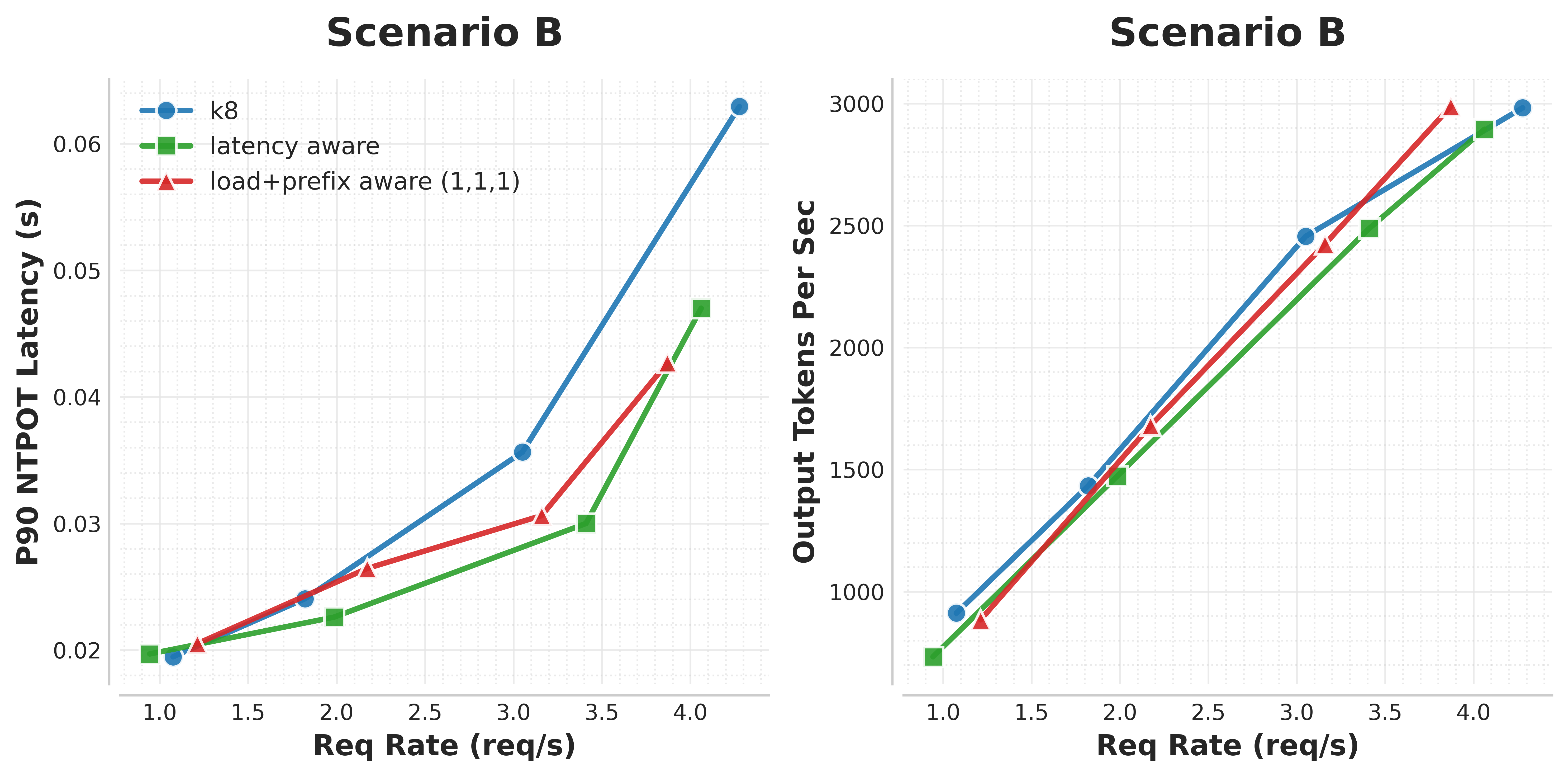
B. Shared Prefix -- Moderate System Prompt Overlap, No System Cache Pressure	This workload also represents a regime where shared system prefixes amortize extremely well. However user context grows faster than workload A leading to onset of prefix cache evictions at a lower QPS.	num_groups=6 num_prompts_per_group=1000 system_prompt_len=1000 question_len=3000 +/- 900 output_len=1000 +/- 300 enable_multi_turn_chat=true	Predicted Latency Scorer
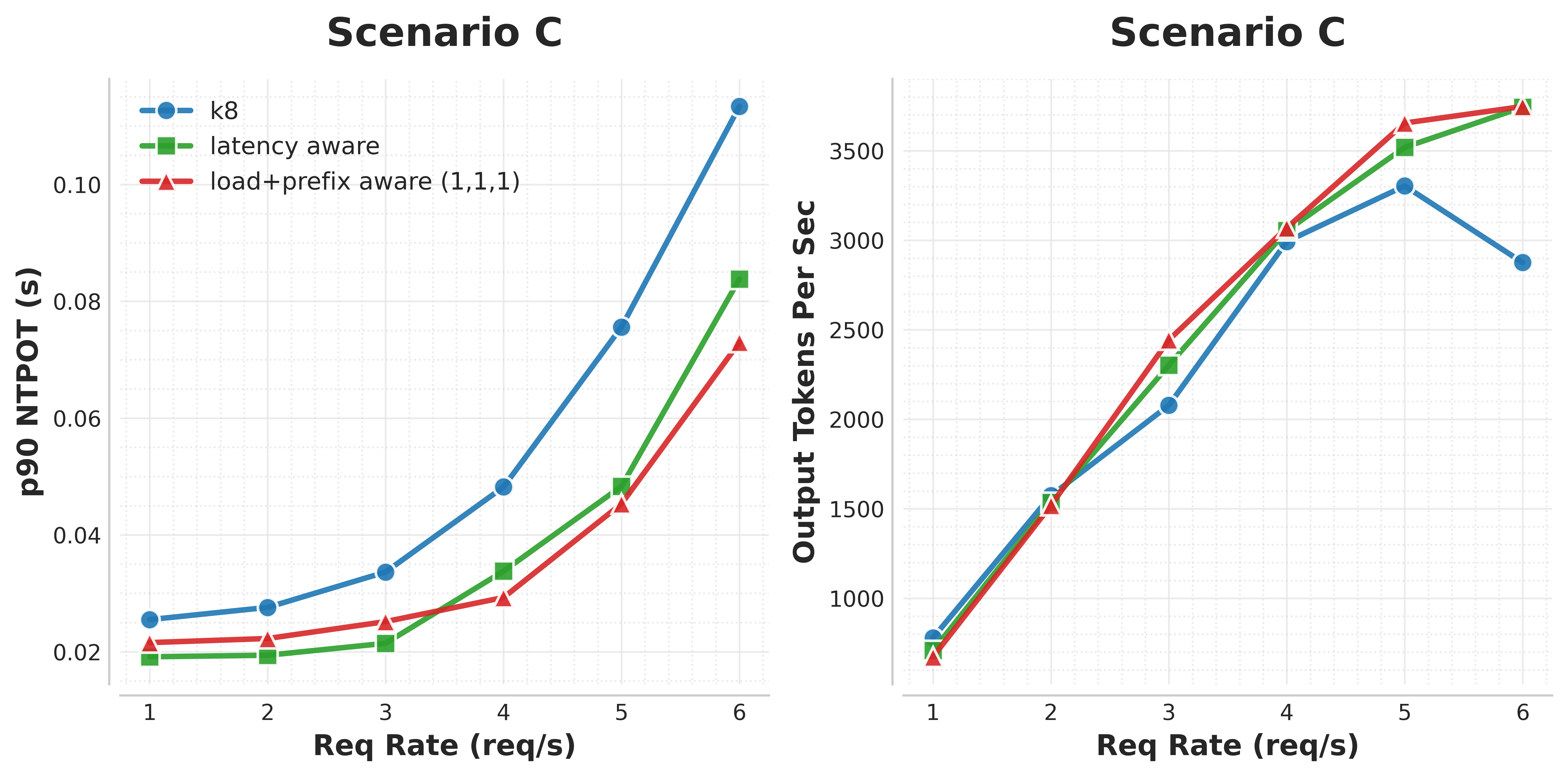
C. Shared Prefix -- Low System Prompt Overlap, High System Cache Pressure	In this workload large system prompts fail to amortize due to low reuse, quickly consuming cache capacity. System-prefix eviction destroys shared reuse, leading to abrupt performance degradation across users.	num_groups=150 num_prompts_per_group=5 system_prompt_len=6000 question_len=1200 +/- 360 output_len=1000 +/- 300 enable_multi_turn_chat=true	Comparable
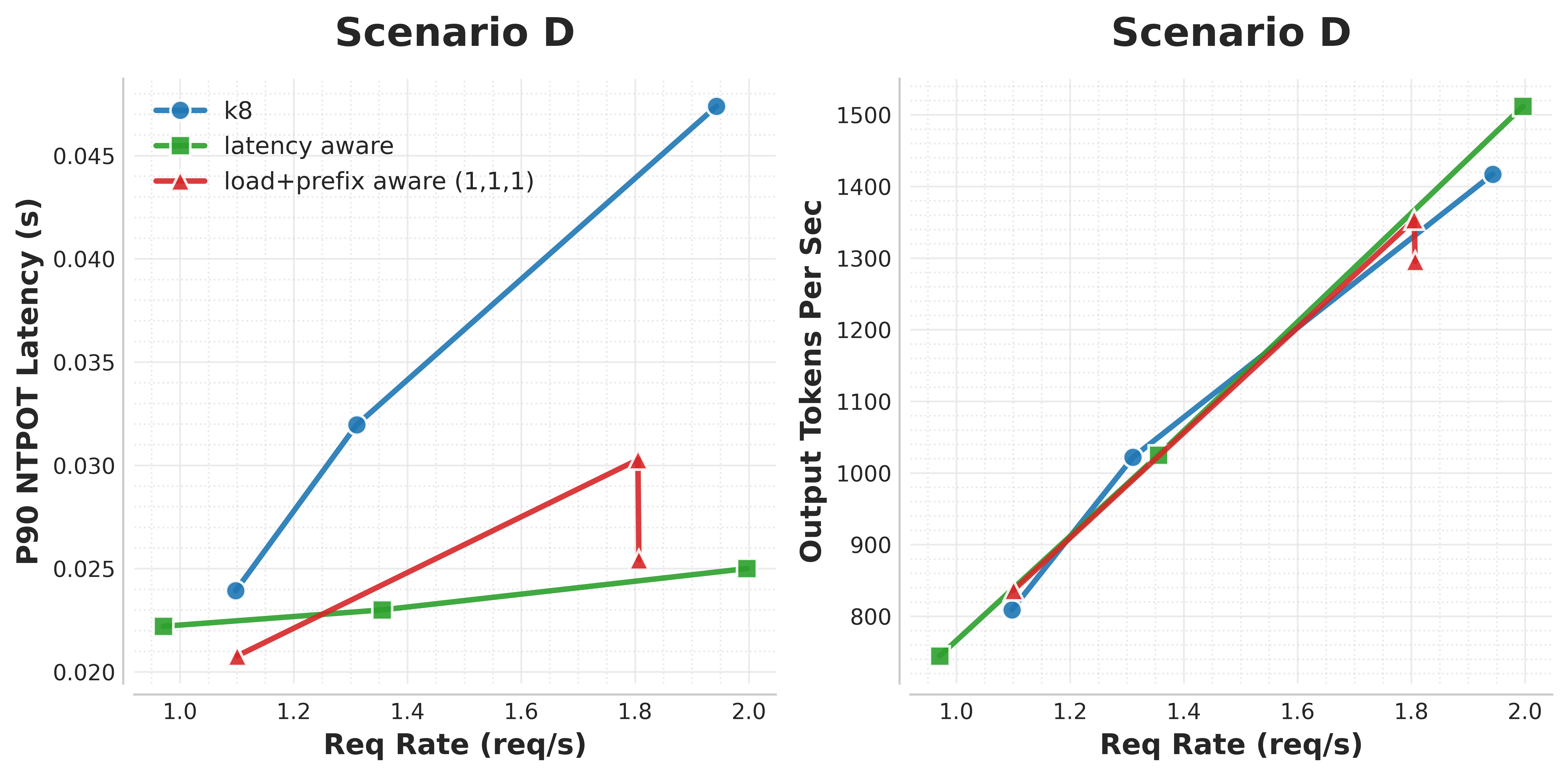
D. Shared Prefix -- Low System Prompt Overlap, Low System Cache Pressure	In this workload, like in workload C, system prompts fail to amortize due to low reuse. But smaller system prompts relative to user prompts ensure that performance is dominated by per-request computation rather than system cache.	num_groups=150 num_prompts_per_group=5 system_prompt_len=1000 question_len=6200 +/- 1860 output_len=1000 +/- 300 enable_multi_turn_chat=true	Predicted Latency Scorer
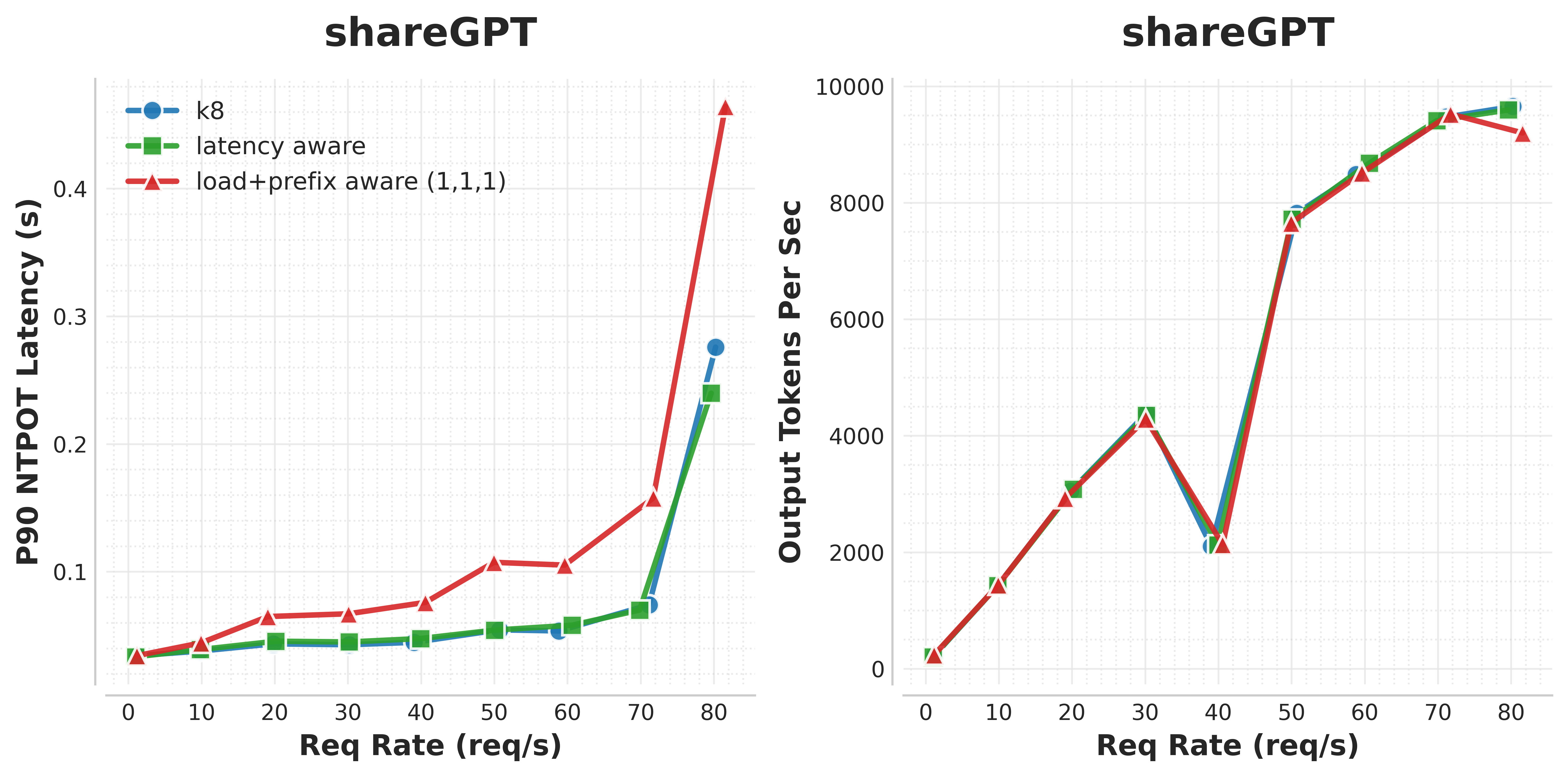
ShareGPT	A chatbot-style workload with minimal prefix overlap across prompts.		Predicted Latency Scorer

---

Results

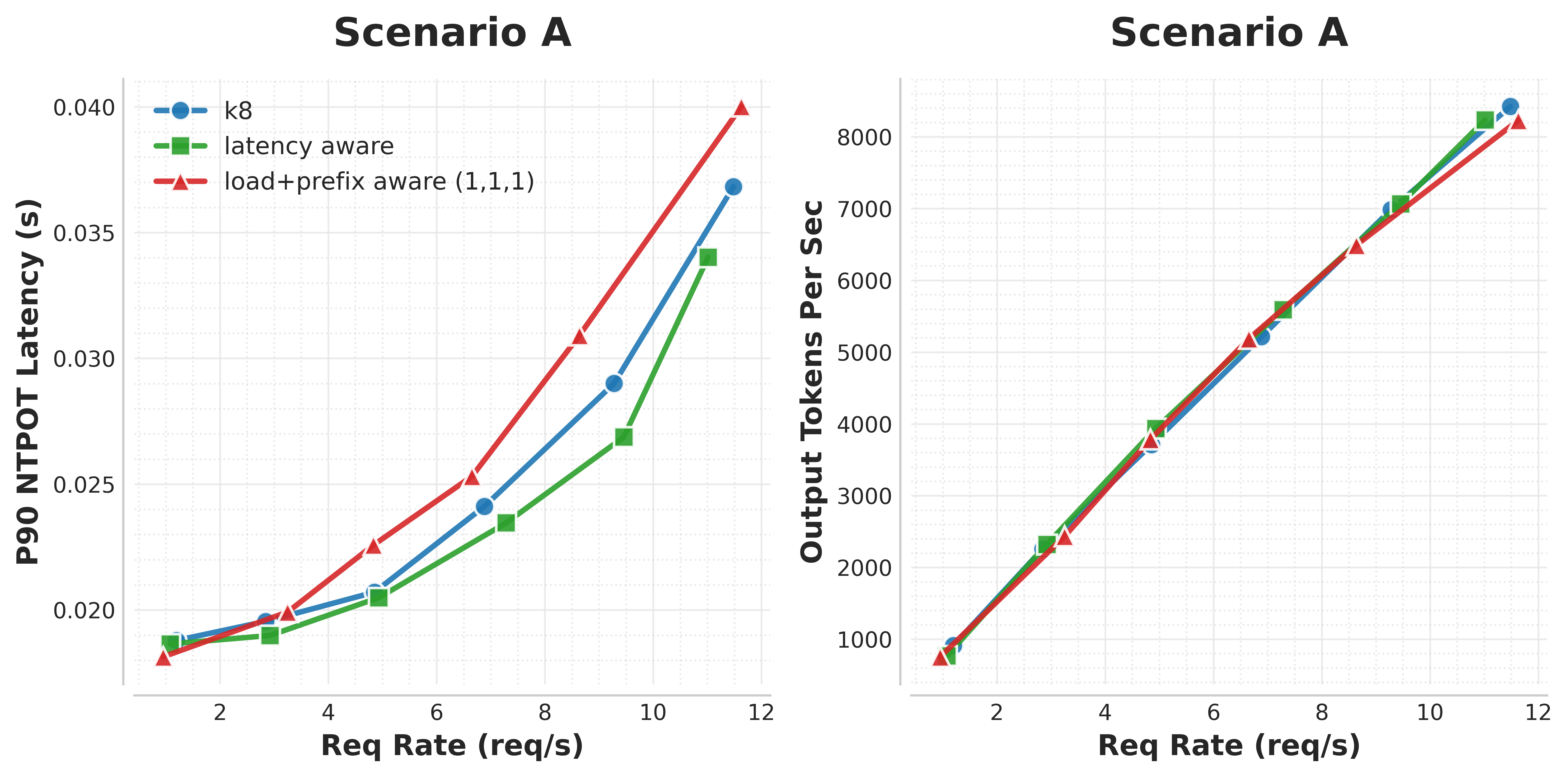
Below we compare different load balancing strategies across the four scenarios above and the ShareGPT dataset. In every scenario, the QPS is increased until throughput saturation occurs and queues begin to form. At each point, requests are sent for 100 seconds, and we wait for their completion before moving on to the next QPS. No SLOs were assumed; the predicted latency scorer simply selects pods with lower predicted latency.

The charts show two metrics: NTPOT (Normalized Time Per Output Token — E2E Latency divided by output length to make it comparable across requests of different output lengths), and output tokens per sec.

In Scenarios A and B, where system cache is amortized across pods, the predicted latency scorer performs best. In Scenario D, which has some system cache churn but user prompts much larger than system prompts, the predicted latency scorer performs as well as the load+prefix aware routing with weights (1, 1, 1). In Scenario C, which has very high system cache churn, the predicted latency scorer performs comparably to load+prefix aware scorers, while still outperforming standard Kubernetes load balancing. In this scenario, performance is governed by discrete cache-eviction events rather than gradual saturation, whereas the latency predictor's greedy routing strategy is inherently better suited to modeling continuous resource contention, such as queueing and KV-cache utilization. Alternate prefix distribution strategies could further improve performance in high-churn scenarios. For instance, pinning critical KV cache prefixes (like system prompts in this case) ensures they remain non-evictable. Similarly, using a no-hit-lru-scorer can improve performance by intelligently distributing "cold" requests to prevent hotspots during the formation of new prefix-caches.

Overall, predicted-latency aware routing consistently performs as well as or better than standard Kubernetes routing and load+prefix-aware routing in all tested scenarios, while eliminating the need for manual parameter tuning.

Production Workload

In addition to the synthetic scenarios above, we evaluated against a workload derived from real production traffic at an internal Google service. The benchmarking profile was constructed from 7 days of traffic serving a large open model via vLLM, analyzing input token counts, output token counts, request rates, and prefix cache hit rates. The resulting profile represents the median (p50) production request.

This workload exhibits the characteristics discussed in the introduction: high variance in both input token counts (mean 729, std 13550, max 131072) and output token counts (mean 300, std 2213, max 8192), along with high but unstable prefix cache reuse (~94% at peak, with frequent collapses). This makes it a strong test of whether routing strategies can adapt to rapidly shifting traffic patterns.

Benchmark Configuration

• Model: Qwen3-480B on vLLM
• Hardware: 13 servers, each with 8x NVIDIA H200 GPUs
• Traffic shape: 8-stage load ladder alternating between 1.0 and 5.0 RPS to simulate realistic traffic spikes
• Request distribution: system_prompt_len=1000, question_len=729 +/- 13550, output_len=300 +/- 2213, multi_turn=true
• Cache hit rate: ~94% (matching production peak)
• Load type: Poisson distribution with concurrency limit of 1000

Routing Strategies Compared

Strategy	Description
No Gateway	Direct connection to model servers (k8s round-robin baseline)
Old Params (111)	Load+prefix scorer with weights (1, 1, 1)
New Params (322)	Load+prefix scorer with tuned weights (3, 2, 2)
Latency Prediction	Predicted-latency based routing, replacing all heuristic scorers

Results

Scenario	Success Rate	E2E p50	E2E p95	TTFT p50	TTFT p95	TPOT p50	TPOT p99
No Gateway	~99.8%	15.98s	38.85s	4.47s	24.04s	35ms	93ms
Load + Prefix (111)	~99.9%	16.42s	35.06s	2.86s	18.06s	39ms	103ms
Load + Prefix (322)	100%	13.42s	26.55s	3.38s	16.78s	28ms	63ms
Latency Prediction	~99.9%	9.06s	22.57s	0.97s	11.34s	22ms	53ms

Latency prediction delivers the lowest latency across all metrics:

• E2E latency: 9.06s p50 (43% lower than the best heuristic-based approach) and 22.57s p95 (15% lower)
• TTFT: 0.97s p50 (70% lower than the best heuristic) and 11.34s p95 (32% lower)
• TPOT: 22ms p50 and 53ms p99, the lowest across all strategies

The improvement is most pronounced at the high-load stages (stages 3, 5, 7), where latency prediction consistently stays well below all other strategies.

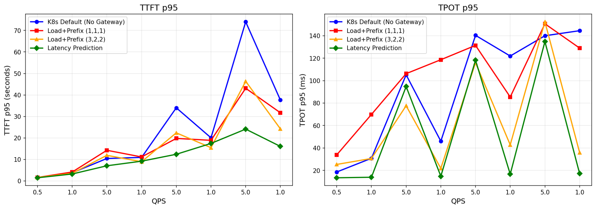
These results are particularly notable because the Load+Prefix (3,2,2) weights were specifically tuned for this workload based on analysis of the production traffic profile. Latency prediction outperforms it -- and all other heuristic-based approaches -- without any workload-specific tuning.

Prediction Server Scalability

At high replica counts, the EPP issues one prediction call per candidate pod per incoming request, so prediction QPS scales with both request rate and cluster size. At each QPS level in the table below, we assume 100 model server endpoints, so the prediction server is generating predictions for all 100 pods per request. To handle this, the Go sidecar coalesces concurrent EPP prediction requests within a 1ms window into a single batched HTTP call, and load-balances across multiple prediction server instances -- each running 28 uvicorn workers. Latency scales roughly linearly with QPS, and adding a prediction server adds 28 cores of inference capacity.

QPS	Avg (ms)	p50 (ms)	p99 (ms)	p99.9 (ms)	Prediction Servers
1	15.7	15	25	25	1
10	13.5	13	18	46	1
100	12.8	12	16	46	1
1,000	15.0	15	26	49	1
2,500	~19	~17	~36	~65	1
5,000	~27	~23	~74	~99	2
7,500	~35	~30	~96	~137	3
10,000	~48	~40	~137	~189	4

5-minute stability test at each level. Each prediction server runs 28 uvicorn workers on a C4 machine (28 cores). All runs achieved 100% success rate.

Try It: A Well-Lit Path

Prereqs

• Install the Inference Gateway extension with the latency prediction sidecars: https://gateway-api-inference-extension.sigs.k8s.io/guides/latency-based-predictor/

Smoke test

1. Health checks

kubectl get pods
curl http://<pod-ip>:8000/readyz   # training
curl http://<pod-ip>:8001/readyz   # prediction (and 8002, 8003, ...)
# EPP health on 9003

2. Send an SLO-aware request

curl -v $GW_IP/v1/completions \
  -H 'Content-Type: application/json' \
  -H 'x-prediction-based-scheduling: true' \
  -H 'x-slo-ttft-ms: 200' \
  -H 'x-slo-tpot-ms: 50' \
  -d '{
    "model": "Qwen/Qwen3-32B",
    "prompt": "what is the difference between Franz and Apache Kafka?",
    "max_tokens": 200,
    "temperature": 0,
    "stream_options": {"include_usage": "true"},
    "stream": "true"
  }'

3. Watch the picker think (EPP logs, -v=4)

msg:"Running profile handler, Pick profiles" plugin:"slo-aware-profile-handler/slo-aware-profile-handler"
msg:"Before running scorer plugins" pods:[{... "pod_name":"...-5k7qr"}, {... "pod_name":"...-9lp5g"}]
msg:"Pod score" scorer_type:"slo-scorer" pod_name:"vllm-...-9b4wt" score:0.82
msg:"Picked endpoint" scorer_type:"slo-scorer" selected_pod:"vllm-...-9b4wt"

---

Tradeoffs & Gaps

The following areas highlight current limitations and ongoing work for the Predicted-Latency Aware Scheduling system:

• Addressing Homogeneous Pool Assumptions Current models assume uniform serving pods regarding GPU types and runtimes. Future updates will incorporate richer features and per-variant training to better support heterogeneous pools.

Takeaway

Accelerator performance is fairly predictable when we account for both the current model server GPU state and request characteristics. By applying online machine learning with a narrow horizon, we can train a model that avoids overfitting while staying accurate to changing workloads. With a good predictor in place, we can route requests based on expected latency, leading to smarter and more efficient load balancing.

---

Get Involved

• Docs & guides: https://gateway-api-inference-extension.sigs.k8s.io/guides/latency-based-predictor/

Appendix

Multi-Turn Cache Capacity Analysis

Theoretical Capacity Estimates

This analysis evaluates what percentage of user and system prompts can be prefix cached assuming perfect load balancing. Assuming 10 pods (H100 80 GB), the total cluster capacity is ~5,120,000 tokens.

Multi-Round Context Assumptions:

• We assume a multi-turn chat scenario where the conversation context grows cumulatively.
• For every round, the previous question AND the previous model response are appended to the context of the next question.
• To satisfy a 5-turn session, the cache must hold the "Working Set" for 4 rounds (the accumulated history of Turns 1-4 serves as the prefix for Turn 5).
• The calculation assumes that System Prompts are prioritized and pinned in the cache. User history is only allocated space from the remaining capacity after all unique system prompts for the active groups are stored.

Key Variables:

• Total Capacity: 32000 blocks * 16 tokens * 10 pods = 5,120,000 tokens
• Unique Sys Tokens: #Groups * System Prompt Tokens
• Unique User Tokens (4 Rounds): #Users * (User Prompt Tokens + Output Len) * 4

Workload	Groups	Users Per Group	Sys Prompt Tokens	User Prompt Tokens	Output Len	Total Unique Sys Tokens	Total Rounds	Total Unique User Tokens (1 round)	Total Cache Capacity	% sys prompts fit	% user prompts fit
A	6	1,000	1,000	30	1,000	6,000	4	24,720,000	5,120,000	100.00%	20.69%
B	6	1,000	1,000	3,000	1,000	6,000	4	96,000,000	5,120,000	100.00%	5.33%
C	150	5	6,000	1,200	1,000	900,000	4	6,600,000	5,120,000	100.00%	63.94%
D	150	5	1,000	6,200	1,000	150,000	4	21,600,000	5,120,000	100.00%	23.01%

We notice that we have theoretically enough capacity to store the system prompts, however as we shall see below what also matters is the ratio between user and system prompts that determines the cache eviction dynamics.

KV Cache Behavior Across Workloads A-D

This section analyzes how workload inputs shape cache behavior, and manifests in prefix reuse, cache pressure, and eviction dynamics using a simple event based simulation.

Each workload varies six core inputs:

• System prompt size (system_prompt_len)
• Prefix sharing structure (num_groups each with a unique system prompt and num_prompts_per_group signifying number of users per group)
• User context growth (enable_multi_turn_chat) If turned on, each user appends its prompt to its previous prompts and responses.
• Request shape (question_len, output_len)

The simulation produces the figures below that should be read as answering four questions:

• How much of the system prompt and user prompt is typically reused?
• How quickly does cache pressure build under load?
• When evictions occur, what is being evicted?
• At what QPS do evictions occur?

Here we assume a single model server running on a 2 x H100 80 GB pod (TP=2). The requests are sent at different QPS for a fixed duration (100 secs).

Note: We assume cache creation and eviction is instantaneous; in reality, it depends on the prefill and decode times which we are not simulating. So effectively, in this simulation, QPS functions only as a proxy for the total number of prompts processed, ignoring the concurrency overhead that actual QPS imposes. Thus, in practice, the actual onset of cache eviction can be much earlier than what the simulation suggests. For example, in Scenario A, we see the onset of cache eviction happen around QPS = 14 with 10 pods (which roughly translates to QPS = 1.4 with 1 pod) experimentally, whereas the theoretical results below indicate a higher threshold. For other scenarios, the theoretical cache eviction QPS matches closely with what we observed experimentally.

---

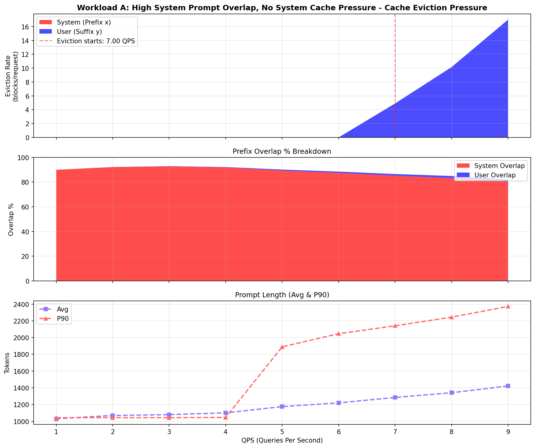
Workload A -- High System Prompt Overlap, No System Cache Pressure

Inputs

• Structure: Few groups, many users per group (6 groups, 1000 users per group).
• Shape: Large system prompt relative to user prompt (1000:30 ratio).
• Context: Multi-turn enabled.
• Variance: 30% variance in user prompt and output length.

Interpretation Workload A represents a regime where shared system prefixes amortize extremely well, and user context grows slowly enough that cache pressure remains low.

---

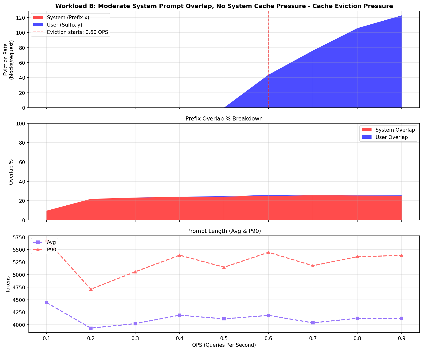
Workload B -- Moderate System Prompt Overlap, No System Cache Pressure

Inputs

• Structure: Few groups, many users per group (6 groups, 1000 users per group).
• Shape: Smaller system prompt relative to user prompt (1000:3000 ratio).
• Context: Multi-turn enabled.
• Variance: 30% variance in user prompt and output length.

Interpretation Although this workload benefits from strong system reuse, longer user turns accelerate user context growth. Importantly, cache degradation is localized: user-block eviction preserves shared prefixes, preventing a global collapse in reuse.

---

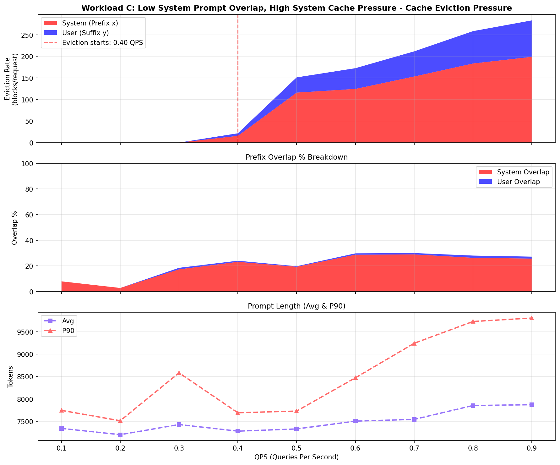
Workload C -- Low System Prompt Overlap, High System Cache Pressure

Inputs

• Structure: Many groups, few users per group (150 groups, 5 users per group).
• Shape: Large system prompt relative to user prompt (6000:1200 ratio).
• Context: Multi-turn enabled.
• Variance: 30% variance in user prompt and output length.

Interpretation In Workload C, large system prompts fail to amortize due to low reuse, quickly consuming cache capacity. System-prefix eviction destroys shared reuse, leading to abrupt performance degradation across users.

---

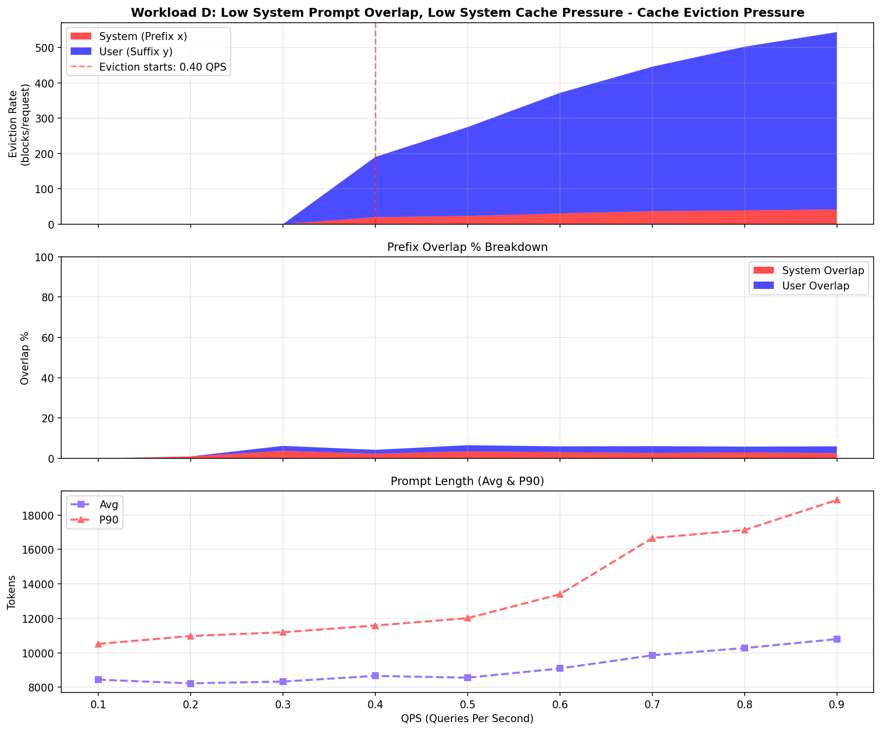
Workload D -- Low System Prompt Overlap, Low System Cache Pressure

Inputs

• Structure: Many groups, few users per group (150 groups, 5 users per group).
• Shape: Moderate system prompt with very large user questions. (1000:6200 ratio)
• Context: Multi-turn enabled.
• Variance: 30% variance in user prompt and output length.

Interpretation In Workload D, cache overlap is low because of many groups. But smaller system prompts relative to user prompts ensure that performance is dominated by per-request computation rather than cache churn.

---

Summary

Metric	Workload A	Workload B	Workload C	Workload D
Prompt Reuse	High (~80%)	Moderate (~20%)	Low (~10%)	Very Low (5%)
Eviction Onset QPS	7	0.6	0.4	0.4
Eviction Target	User History	User History	System Prompts	Mix of user history and system prompts though largely dominated by user prompt
Best Scheduling Strategy	Latency Aware Scheduling	Latency Aware Scheduling	Comparable	Latency Aware